Seminar 1. EEG analysis

Seminar 1. EEG analysis#

Plan

Read and visualize the data
Preprocess the data
Use ICA for noise reduction
Compute ERP and plot topomaps for ERP
Compute beta band envelopes for ERP
Compute coherence

Part 1#

All preprocessing and some data analysis of EEG data can be done using the Python library MNE.

# For Colab only
# !pip install mne
# !pip install mne-connectivity

import warnings
warnings.filterwarnings('ignore')
import mne
import numpy as np
import pandas as pd
import matplotlib.pyplot as plt
import matplotlib
import seaborn as sns
import mne_connectivity

# not in colab
%matplotlib notebook
# in colab
# %matplotlib inline

mne.io includes the funtions for different EEG-record formats: https://mne.tools/stable/documentation/implementation.html#supported-data-formats

We will work with data for one patient from EEG Motor Movement/Imagery Dataset.

# !wget "https://www.physionet.org/files/eegmmidb/1.0.0/S003/S003R03.edf"

# !wget "https://www.physionet.org/files/eegmmidb/1.0.0/S003/S003R03.edf.event"

# !ls

sample = mne.io.read_raw_edf('S003R03.edf', verbose=False, preload=True)

Get some info about a record

sample.info

General

Measurement date	August 12, 2009 16:15:00 GMT
Experimenter	Unknown
Participant	X

Channels

Digitized points	Not available
Good channels	64 EEG
Bad channels	None
EOG channels	Not available
ECG channels	Not available

Data

Sampling frequency	160.00 Hz
Highpass	0.00 Hz
Lowpass	80.00 Hz

# Sampling frequency
sample.info['sfreq']

160.0

# Length in seconds
len(sample) / sample.info['sfreq']

125.0

# Number of channels
len(sample.ch_names)

Channel selection and adding a montage#

sample.ch_names[:3]

['Fc5.', 'Fc3.', 'Fc1.']

# fix trailing dots in channel names
# use sample.rename_channels(map)

# YOUR CODE HERE
map = {}
for ch in sample.ch_names:
    map[ch] = ch.replace(".", "")
sample.rename_channels(map)

General

Measurement date	August 12, 2009 16:15:00 GMT
Experimenter	Unknown
Participant	X

Channels

Digitized points	Not available
Good channels	64 EEG
Bad channels	None
EOG channels	Not available
ECG channels	Not available

Data

Sampling frequency	160.00 Hz
Highpass	0.00 Hz
Lowpass	80.00 Hz
Filenames	S003R03.edf
Duration	00:02:05 (HH:MM:SS)

sample.ch_names[:3]

['Fc5', 'Fc3', 'Fc1']

# 19 channels from International 10-20 system. no A1 and A2 here
# Be careful. Pure 10-20 labeling differs from high-resolution montages
# In MNE, 10-20 montage is actually an extended high-resulution version of 10-20
# FYI, mapping from pure 10-20 to high-resolution versions
# T3 = T7
# T4 = T8
# T5 = P7
# T6 = P8

channels_to_use = [
    # prefrontal
    'Fp1',
    'Fp2',
    # frontal
    'F7',
    'F3',
    'F4',
    'Fz',
    'F8',
    # central and temporal
    'T7',
    'C3',
    'Cz',
    'C4',
    'T8',
    # parietal
    'P7',
    'P3',
    'Pz',
    'P4',
    'P8',
    # occipital
    'O1',
    'O2',
]

sample_1020 = sample.copy().pick(channels_to_use)

# check that everything is OK
assert len(channels_to_use) == len(sample_1020.ch_names)

ten_twenty_montage = mne.channels.make_standard_montage('standard_1020')
len(ten_twenty_montage.ch_names)

sample_1020.set_montage(ten_twenty_montage)

General

Measurement date	August 12, 2009 16:15:00 GMT
Experimenter	Unknown
Participant	X

Channels

Digitized points	22 points
Good channels	19 EEG
Bad channels	None
EOG channels	Not available
ECG channels	Not available

Data

Sampling frequency	160.00 Hz
Highpass	0.00 Hz
Lowpass	80.00 Hz
Filenames	S003R03.edf
Duration	00:02:05 (HH:MM:SS)

sample_1020.plot_sensors(show_names=True);

Explore the signals#

sample_1020.compute_psd().plot();

Effective window size : 12.800 (s)

Plotting power spectral density (dB=True).

Do you see peaks connected to power line noise?

The notch filter’s purpose is to filter out activity at a specific frequency (rather than a frequency range). Because the alternating current in standard electric outlets in North America oscillates at 60 Hz, electric fields produced by the 60-Hz activity in the environment that surrounds us in our indoor environments frequently contaminates the EEG. Sixty-hertz notch filters (filters designed specifically to filter out 60-Hz activity) are used to attenuate or eliminate this unwanted signal. In countries where line frequencies are 50 Hz, 50-Hz notch filters are used for the same purpose.

Band-pass filtering#

It’s better to remove low-freq components < 1 Hz and high-freq > 50Hz (non-informative for EEG)

Let’s use IIR filter.

sample_1020.filter(l_freq=1, h_freq=50, method='iir')

Filtering raw data in 1 contiguous segment

Setting up band-pass filter from 1 - 50 Hz

IIR filter parameters

---------------------

Butterworth bandpass zero-phase (two-pass forward and reverse) non-causal filter:

- Filter order 16 (effective, after forward-backward)

- Cutoffs at 1.00, 50.00 Hz: -6.02, -6.02 dB

General

Measurement date	August 12, 2009 16:15:00 GMT
Experimenter	Unknown
Participant	X

Channels

Digitized points	22 points
Good channels	19 EEG
Bad channels	None
EOG channels	Not available
ECG channels	Not available

Data

Sampling frequency	160.00 Hz
Highpass	1.00 Hz
Lowpass	50.00 Hz
Filenames	S003R03.edf
Duration	00:02:05 (HH:MM:SS)

# Plot psd after filtering

# YOUR CODE HERE

Plot EEG signals#

sample_1020.plot(n_channels=8, duration=20);

Using matplotlib as 2D backend.

# Plot in better scale. Use 'scalings' argument

# YOUR CODE HERE
sample_1020.plot(n_channels=8, duration=20, scalings=3e-4);

Extracting events#

Mne has several functions for event selection.

mne.find_events is used when events are stored in trigger channels (e.g. FIFF format)
mne.events_from_annotations is used for when events are stored in annotations (EDF+ format)

Look for documentation for your EEG-record format

Here we have EDF+ format

events, events_dict = mne.events_from_annotations(sample_1020)

Used Annotations descriptions: ['T0', 'T1', 'T2']

events_dict

{'T0': 1, 'T1': 2, 'T2': 3}

events[:5]

array([[   0,    0,    1],
       [ 672,    0,    3],
       [1328,    0,    1],
       [2000,    0,    2],
       [2656,    0,    1]])

Epochs objects are a data structure for representing and analyzing equal-duration chunks of the EEG/MEG signal. Epochs are most often used to represent data that is time-locked to repeated experimental events. The Raw object and the events array are the bare minimum needed to create an Epochs object, which we create with the mne.Epochs class constructor.

However, you will almost surely want to change some of the other default parameters. Here we’ll change tmin and tmax (the time relative to each event at which to start and end each epoch).

epochs = mne.Epochs(sample_1020, events,  tmin=-0.5, tmax=0.8, preload=True)

Not setting metadata

30 matching events found

Setting baseline interval to [-0.5, 0.0] s

Applying baseline correction (mode: mean)

0 projection items activated

Using data from preloaded Raw for 30 events and 209 original time points ...

1 bad epochs dropped

pd.DataFrame(epochs.events, columns=['_', '__', 'event_id'])['event_id'].value_counts()

event_id
1    14
3     8
2     7
Name: count, dtype: int64

Check that length is right

for epoch in epochs:
    break
epoch.shape

(19, 209)

epoch.shape[1] / sample_1020.info['sfreq']

1.30625

sample_1020.to_data_frame().shape

(20000, 20)

df = epochs.to_data_frame()
df.head(3).iloc[:, :10]

	time	condition	epoch	Fp1	Fp2	F7	F3	F4	Fz	F8
0	-0.50000	3	1	236.675891	244.275703	125.936913	88.829681	112.445086	73.438632	145.805904
1	-0.49375	3	1	175.970007	183.425016	103.803572	63.009365	82.687750	48.730906	115.749079
2	-0.48750	3	1	127.095181	132.985975	61.669835	31.478465	62.299189	33.384794	93.870855

df[sample_1020.ch_names + ['epoch']].groupby('epoch').agg(lambda arr: arr.max() - arr.min()).hist(figsize=[10, 10]);
plt.tight_layout()

Note also that the Epochs constructor accepts parameters reject for rejecting individual epochs based on signal amplitude.

epochs = mne.Epochs(sample_1020, events,  tmin=-0.5, tmax=0.8, reject={'eeg': 600e-6}, preload=True, baseline=(-.1, 0))

Not setting metadata

30 matching events found

Applying baseline correction (mode: mean)

0 projection items activated

Using data from preloaded Raw for 30 events and 209 original time points ...

    Rejecting  epoch based on EEG : ['Fp1', 'Fp2']

    Rejecting  epoch based on EEG : ['Fp2']

    Rejecting  epoch based on EEG : ['Fp2']

    Rejecting  epoch based on EEG : ['Fp2']

    Rejecting  epoch based on EEG : ['Fp2']

    Rejecting  epoch based on EEG : ['Fp1', 'Fp2']

    Rejecting  epoch based on EEG : ['Fp1', 'Fp2']

    Rejecting  epoch based on EEG : ['Fp1', 'Fp2']

    Rejecting  epoch based on EEG : ['Fp1', 'Fp2']

    Rejecting  epoch based on EEG : ['Fp1', 'Fp2']

    Rejecting  epoch based on EEG : ['Fp2']

    Rejecting  epoch based on EEG : ['Fp1', 'Fp2']

    Rejecting  epoch based on EEG : ['Fp1', 'Fp2']

    Rejecting  epoch based on EEG : ['Fp1', 'Fp2']

15 bad epochs dropped

PSD on epochs differs from the raw. More averaging is used

epochs.plot_psd();

NOTE: plot_psd() is a legacy function. New code should use .compute_psd().plot().

    Using multitaper spectrum estimation with 7 DPSS windows

Plotting power spectral density (dB=True).

Averaging across epochs...

epochs.plot(n_channels=8, scalings={'eeg':3e-4});

epochs.event_id

{'1': 1, '2': 2, '3': 3}

# check number of events of each type
# use epochs.events

# Your code here

evoked_T0 = epochs['1'].average()
evoked_T1 = epochs['2'].average()
evoked_T2 = epochs['3'].average()

evoked_T0.plot(spatial_colors=True);

evoked_T1.plot(spatial_colors=True);

evoked_T2.plot(spatial_colors=True);

Part 2#

Independent Component Analysis for Artifact Removal#

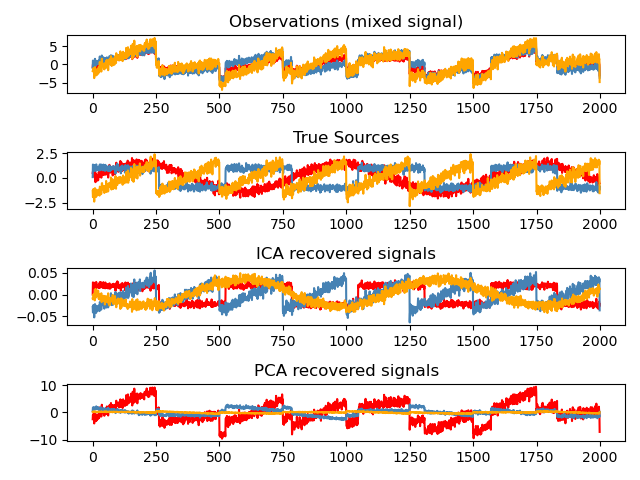
Independent component analysis (ICA) is used to estimate sources given noisy measurements. Imagine 3 instruments playing simultaneously and 3 microphones recording the mixed signals. ICA is used to recover the sources ie. what is played by each instrument.

ICA can be used for artifact repair in EEG data. We denote an “artifact” as any component of the EEG signal that is not directly produced by human brain activity.

Types of EEG artifacts#

The ability to recognize artifacts is the first step in removing them. EEG artifacts can be classified depending on their origin, which can be physiological or external to the human body (non-physiological). The most usual are:

Physiological artifacts:

Ocular activity
Muscle activity
Cardiac activity
Perspiration
Respiration

Non-physiological / Technical artifacts:

Electrode pop
Cable movement
Incorrect reference placement
AC electrical and electromagnetic interferences
Body movements

More information can be found via links:

ica = mne.preprocessing.ICA(n_components=12, random_state=42)

ica.fit(sample_1020)

Fitting ICA to data using 19 channels (please be patient, this may take a while)

Selecting by number: 12 components

Fitting ICA took 0.4s.

Method	fastica
Fit parameters	algorithm=parallel fun=logcosh fun_args=None max_iter=1000
Fit	27 iterations on raw data (20000 samples)
ICA components	12
Available PCA components	19
Channel types	eeg
ICA components marked for exclusion	—

Using get_explained_variance_ratio(), we can retrieve the fraction of variance in the original data that is explained by our ICA components in the form of a dictionary:

explained_var_ratio = ica.get_explained_variance_ratio(sample_1020)
for channel_type, ratio in explained_var_ratio.items():
    print(f"Fraction of {channel_type} variance explained by all components: {ratio}")

Fraction of eeg variance explained by all components: 0.9853007875511103

ica.plot_sources(sample_1020);

Creating RawArray with float64 data, n_channels=12, n_times=20000

    Range : 0 ... 19999 =      0.000 ...   124.994 secs

Ready.

ica.plot_components();

Inspect ICA components more deeply. Check out spectrogram. Segments info is not very relevant here since we build ICA on the raw data

We expect to see alpha and beta rythms picks on the spectrogram for good components (7-13 Hz and 13-30Hz respectively). And also slight decrease as frequency goes higher

ica.plot_properties(sample_1020, picks=[0]);

    Using multitaper spectrum estimation with 7 DPSS windows

Not setting metadata

62 matching events found

No baseline correction applied

0 projection items activated

# blinks
ica.plot_overlay(sample_1020, exclude=[0,1,2,8]);

Applying ICA to Raw instance

    Transforming to ICA space (12 components)

    Zeroing out 4 ICA components

    Projecting back using 19 PCA components

ica.plot_overlay(sample_1020, exclude=[0, 1, 2, 8], picks=['F3']);

Applying ICA to Raw instance

    Transforming to ICA space (12 components)

    Zeroing out 4 ICA components

    Projecting back using 19 PCA components

ica.exclude = [0,1,2,8]

sample_1020_clr = sample_1020.copy()

ica.apply(sample_1020_clr)

Applying ICA to Raw instance

    Transforming to ICA space (12 components)

    Zeroing out 4 ICA components

    Projecting back using 19 PCA components

General

Measurement date	August 12, 2009 16:15:00 GMT
Experimenter	Unknown
Participant	X

Channels

Digitized points	22 points
Good channels	19 EEG
Bad channels	None
EOG channels	Not available
ECG channels	Not available

Data

Sampling frequency	160.00 Hz
Highpass	1.00 Hz
Lowpass	50.00 Hz
Filenames	S003R03.edf
Duration	00:02:05 (HH:MM:SS)

# plot channels

# YOUR CODE HERE
sample_1020_clr.plot(n_channels=8, duration=20, scalings=3e-4);

epochs = mne.Epochs(sample_1020_clr, events,  tmin=-0.5, tmax=0.8, reject={'eeg': 600e-6}, preload=True, baseline=(-.1, 0))

Not setting metadata

30 matching events found

Applying baseline correction (mode: mean)

0 projection items activated

Using data from preloaded Raw for 30 events and 209 original time points ...

1 bad epochs dropped

evoked_T0 = epochs['1'].average()
evoked_T1 = epochs['2'].average()
evoked_T2 = epochs['3'].average()

evoked_T0.plot(spatial_colors=True);

evoked_T1.plot(spatial_colors=True);

evoked_T2.plot(spatial_colors=True);

Let’s plot Global Field Power (GFP).

GFP is, generally speaking, a measure of agreement of the signals picked up by all sensors across the entire scalp: if all sensors have the same value at a given time point, the GFP will be zero at that time point. If the signals differ, the GFP will be non-zero at that time point. GFP peaks may reflect “interesting” brain activity, warranting further investigation.

mne.viz.plot_compare_evokeds(
    dict(rest=evoked_T0, left=evoked_T1, right=evoked_T2),
    legend="upper left",
    show_sensors="upper right",
);

combining channels using GFP (eeg channels)

combining channels using GFP (eeg channels)

combining channels using GFP (eeg channels)

We can also get a more detailed view of each Evoked object using other plotting methods such as plot_joint or plot_topomap. For both plots we can set time points. However, if we choose times = 'peaks', time points will be chosen automatically by checking for 3 local maxima in Global Field Power (GFP).

evoked_T0.plot_joint()
evoked_T0.plot_topomap(times=[0.0, 0.2, 0.3, 0.4, 0.8]);

No projector specified for this dataset. Please consider the method self.add_proj.

evoked_T1.plot_joint()
evoked_T1.plot_topomap(times=[0.0, 0.2, 0.3, 0.4, 0.8]);

No projector specified for this dataset. Please consider the method self.add_proj.

evoked_T2.plot_joint()
evoked_T2.plot_topomap(times=[0.0, 0.2, 0.3, 0.4, 0.8]);

No projector specified for this dataset. Please consider the method self.add_proj.

Computing functional connectivity#

conn_T1 = mne_connectivity.spectral_connectivity_epochs(epochs['2'], method='coh')

Adding metadata with 3 columns

Connectivity computation...

only using indices for lower-triangular matrix

    computing connectivity for 171 connections

    using t=-0.500s..0.800s for estimation (209 points)

    frequencies: 4.6Hz..79.6Hz (99 points)

    Using multitaper spectrum estimation with 7 DPSS windows

    the following metrics will be computed: Coherence

    computing cross-spectral density for epoch 1

    computing cross-spectral density for epoch 2

    computing cross-spectral density for epoch 3

    computing cross-spectral density for epoch 4

    computing cross-spectral density for epoch 5

    computing cross-spectral density for epoch 6

    computing cross-spectral density for epoch 7

    assembling connectivity matrix

[Connectivity computation done]

def plot_topomap_connectivity_2d(info, con, picks=None, pairs=None, vmin=None, vmax=None, cm=None, show_values=False, show_names=True):
    """
    Plots connectivity-like data in 2d

    Drawing every pair of channels will likely make a mess
    There are two options to avoid it:
    - provide picks
    - provide specific pairs of channels to draw
    """

    # get positions
    _, pos, _, _, _, _, _ = mne.viz.topomap._prepare_topomap_plot(info, 'eeg');

#     if picks is None and pairs is None:
#         picks = info.ch_names

    ch_names_lower = [ch.lower() for ch in info.ch_names]
    if picks:
        picks_lower = [ch.lower() for ch in picks]
    if pairs:
        pairs_lower = [tuple(sorted([ch1.lower(), ch2.lower()])) for ch1, ch2 in pairs]

    rows = []
    for idx1, ch1 in enumerate(ch_names_lower):
        for idx2, ch2 in enumerate(ch_names_lower):
            if ch1 >= ch2:
                continue
            if picks and (ch1 not in picks_lower or ch2 not in picks_lower):
                    continue
            if pairs and (ch1, ch2) not in pairs_lower:
                    continue
            rows.append((
                pos[idx1],
                pos[idx2],
                con[idx1, idx2]
            ))

    if not len(rows):
        raise ValueError('No pairs to plot')

    con_to_plot = np.array([row[2] for row in rows])
    if vmin is None:
        vmin = np.percentile(con_to_plot, 2)
    if vmax is None:
        vmax = np.percentile(con_to_plot, 98)
    norm = matplotlib.colors.Normalize(vmin=vmin, vmax=vmax)

    if cm is None:
        cm = sns.diverging_palette(240, 10, as_cmap=True)

    fig, ax = plt.subplots(figsize=[5, 5])
    mne.viz.utils.plot_sensors(info, show_names=show_names, show=False, axes=ax);
    for row in rows:
        if (row[2] > vmin) and  (row[2] < vmax):
          rgba_color = cm(norm(row[2]))
          plt.plot([row[0][0], row[1][0]], [row[0][1], row[1][1]], color=rgba_color)
          if show_values:
              plt.text((row[0][0] + row[1][0]) / 2,
                      (row[0][1] + row[1][1]) / 2,
                      '{:.2f}'.format(row[2]))

conn_T0 = mne_connectivity.spectral_connectivity_epochs(epochs['1'], method='coh', verbose=False);
conn_T1 = mne_connectivity.spectral_connectivity_epochs(epochs['2'], method='coh', verbose=False);
conn_T2 = mne_connectivity.spectral_connectivity_epochs(epochs['3'], method='coh', verbose=False);

conn_T0.get_data(output="dense").shape

(19, 19, 99)

conn_T0_all = conn_T0.get_data(output="dense")[:, :, 12:20].mean(axis=2)
conn_T0_all = conn_T0_all + conn_T0_all.T

conn_T1_all = conn_T1.get_data(output="dense")[:, :, 12:20].mean(axis=2)
conn_T1_all = conn_T1_all + conn_T1_all.T

conn_T2_all = conn_T2.get_data(output="dense")[:, :, 12:20].mean(axis=2)
conn_T2_all = conn_T2_all + conn_T2_all.T

plot_topomap_connectivity_2d(epochs.info, conn_T0_all, picks=epochs.ch_names, vmin=0.85);

# plot connectivity for T1 and T2
# change vmin such way that you see the difference

# YOUR CODE HERE
plot_topomap_connectivity_2d(epochs.info, conn_T1_all, picks=epochs.ch_names, show_values=True, vmin=0.85);

plot_topomap_connectivity_2d(epochs.info, conn_T2_all, picks=epochs.ch_names, show_values=True, vmin=0.85);

Over the motor cortex, beta waves (12-20 Hz) are associated with the muscle contractions that happen in isotonic movements and are suppressed prior to and during movement changes, with similar observations across fine and gross motor skills.

# calculate coherence in beta band
# plot 5-10 pairs that you are interested in
# using pairs=[('F7', 'F4'), ('O2', 'T7'), ...] in function plot_topomap_connectivity_2d

# YOUR CODE HERE

Seminar 1. EEG analysis

Contents

Seminar 1. EEG analysis#

Part 1#

Channel selection and adding a montage#

Explore the signals#

Band-pass filtering#

Plot EEG signals#

Extracting events#

Part 2#

Independent Component Analysis for Artifact Removal#

Types of EEG artifacts#

Computing functional connectivity#